Essential Tips for Microsoft Excel 2016

Microsoft Excel is the industry standard spreadsheet application. Microsoft Excel 2016 is a vast cornucopia of tools that let you manipulate, organize, analyze, and format data in a spreadsheet. Although Excel has been the lifeblood of many a corporate office, research firm, and financial outfit, Excel can be equally as handy and powerful for everyday users. Whether you are a home user managing a household budget, a small business owner managing inventory or a school teacher taking daily attendance, Excel will make your life easier if you learn to use it. Let’s check out those tips.

1 – Resize Columns and Rows

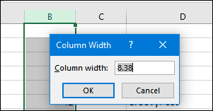
The Excel default cell height and width is hardly one size fits all. Chances are, you’ll need to adjust the column width and row height to accommodate your data. To do that, click the column or row, select the Home tab, then click the Format button within the Cells group. Choose whether you want to adjust the height or width.

Enter the amount then click OK. The column or row should be adjusted to the exact measurement.

You can also manually resize columns and rows using the mouse. Place the mouse pointer between the column or row, click the left mouse button, observe the floating balloon then drag and expand until the desired size is achieved.

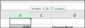
And here’s a handy tip: simply double-click the right border of a column to auto-size the width to the data.

2 – Add or Remove Columns, Rows or Cells

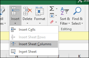
If you need an additional column, row, or cell, you can easily insert it using the Insert and Delete Cells commands. Click the Insert button within the Cells group, then choose the appropriate option.

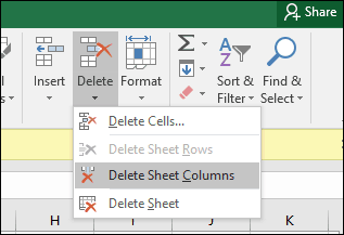
You can also delete a column from within the same group; click the Delete menu, then choose the appropriate action.

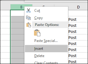
The same action can be performed by right-clicking on the column or cell row.

Learn more about deleting blank cells in Microsoft Excel.

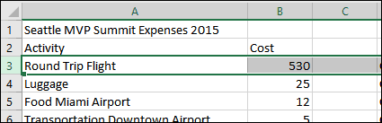
3 – Freeze Panes

If you want to scroll through a spreadsheet without losing focus on a particular part of the sheet or data, the Freeze Panes function is the perfect way to do it. Select the row or column where the data begins in the sheet.

Select the View tab, click the Freeze Panes menu then click Freeze Panes.

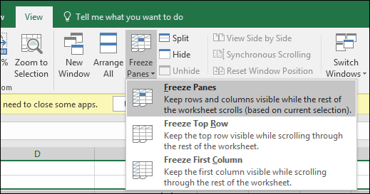
When you scroll, your headings or columns will remain visible.

4 – Change Text Alignment in Cells

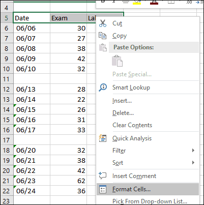
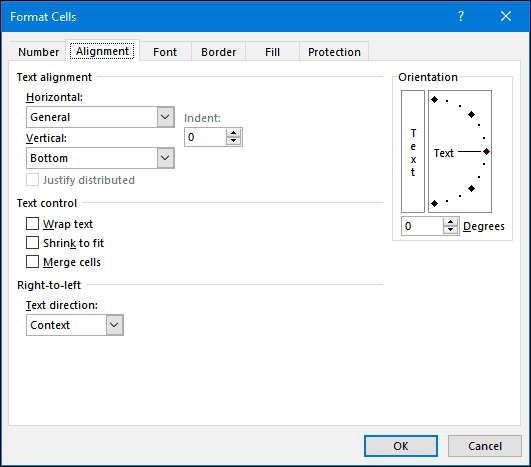
If you need to create a register or labels, you can use the Format Cells dialog to adjust the alignment of text within cells. Select the cells where you would like to apply the formatting, right click on the selection then click Format Cells….

Click the Alignment tab, then use the mouse to change the orientation of the text or enter a value. When satisfied, click OK.

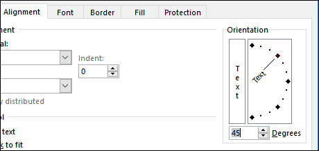
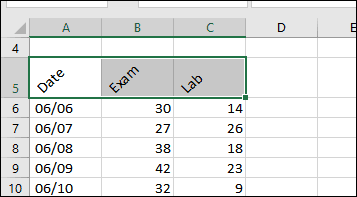
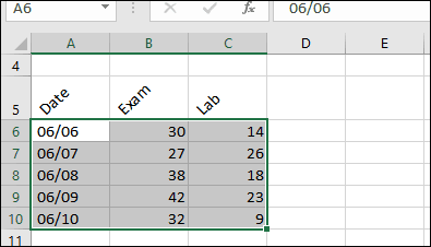
Text within the cells will now appear slanted.

5 – Use Cell Protection to Prevent Editing an Area of the Spreadsheet

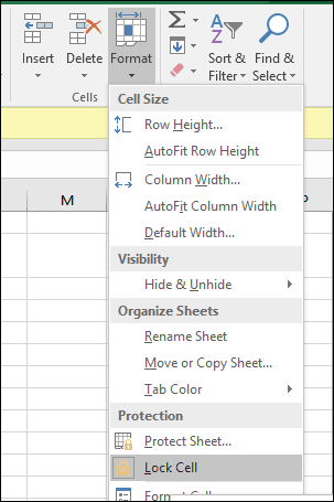
If you share a workbook with other users, it’s important to prevent accidental edits. There are multiple ways you can protect a sheet, but if you just want to protect a group of cells, here is how you do it. First, you need to turn on Protect Sheet. Click the Format menu then click Protect Sheet. Choose the type of modifications you want to prevent other users from making. Enter your password, click OK then click OK to confirm.

Make a selection of the rows or columns you want to prevent other users from editing.

Click the Format menu, then click Lock Cell.

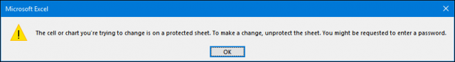
Anytime a user tries to make edits; they will receive the following error message.

To protect an entire spreadsheet, check out our article for instructions about applying encryption and passwords to your Excel spreadsheets and Office files.

6 – Apply Special Formatting to Numbers and Currency in Cells

If you need to apply a specific currency value or determine the decimal place for numbers in your spreadsheet, you can use the Numbers tab within the Formal Cells dialog to do so. Select the numbers you would like to format, right click the selection then select the Numbers tab. Select Currency in the Category list, then choose the number of decimal places and currency format.

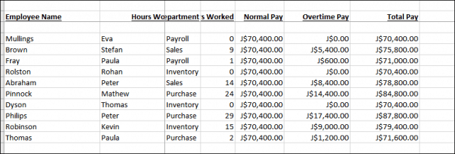
7 – 5 Essential Excel Functions You Should Know – Sum, Average, Max, Min, Count

Excel’s vast true power lies in its functions and formulas. Basic functions let you do quick math operations, while advanced functions let you crunch some serious numbers and perform complex analysis. Just like everyone should know the formatting ropes in Word, you should also know the most popular functions in Excel.

Sum – calculates the total of a range of cells.

Average – calculates the average of a range of cells.

Max – calculates the maximum value in a range of cells.

Min – calculates the minimum value of a range of cells.

Count – calculates the number of values in a range of cells, avoiding empty or cells without numeric data.

Here is how you use a function. Enter the labels for the numbers you would like to produce the calculation for. Select the Function tab, then choose the category of function you would like to apply. Click Insert Function button within the Function Library group or press Shift + F3 on your keyboard. Select the function you need or use the Search for function feature then click OK.

Once you’ve found the function, select it then click OK.

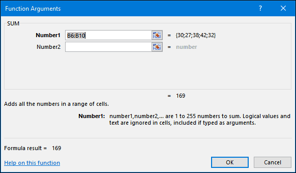
Make any appropriate modifications to the range you are calculating then click OK to apply the function.

8 – Create and Manipulate Charts

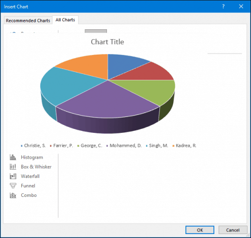
A hallmark feature of Microsoft Excel, creating charts allows you to visually present your well-formed data. Excel makes the process very easy; highlight a range of data in your sheet, select the Insert tab, then click the See all charts button.

Click the All charts tab, then browse the through the list of chart styles.

You can also hover over a sample to see a preview of what the chart will look like. Once satisfied, click OK to insert the chart into the spreadsheet. If you would prefer to keep it in a separate sheet, select the chart, click Move Chart, select New Sheet then click OK.

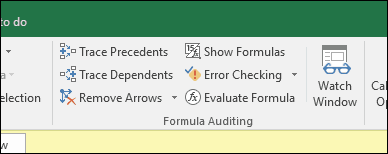
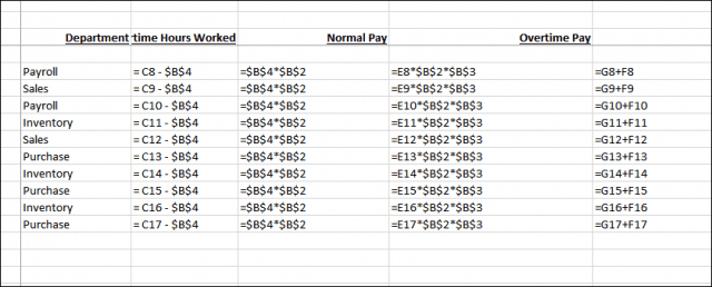
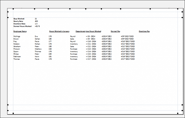
9 – Reveal Formulas

If you want to validate the calculations in your workbook, revealing your formulas is the way to do it.

Select the Formulas tab, then click Show Formulas located in the Formula Auditing group.

Now you can easily check through formulas used in your sheet and also print them. It’s a great way to find errors or to simply understand where the numbers come from.

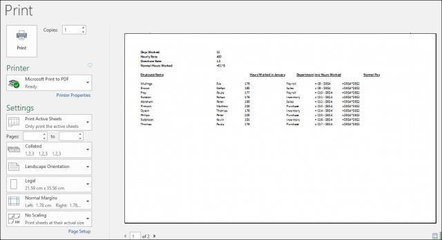
10 – Maximize Printing Options when Printing Large Workbooks

Spreadsheets work great on large widescreen monitors, but sometimes you might need to print out your workbook. If you are not careful, you can end up wasting a lot of paper on something mostly unreadable. Excel takes care of this using the Backstage printing options, which let you adjust the page size and orientation. Spreadsheets are best printed on legal size paper using landscape orientation.

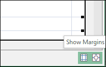
If you need to adjust margins to fit additional information on a single sheet when printing, click the Show Margins button in the right-hand corner of the backstage print tab.

You can then use the margins to adjust the columns to fit any data might spill over to another page.

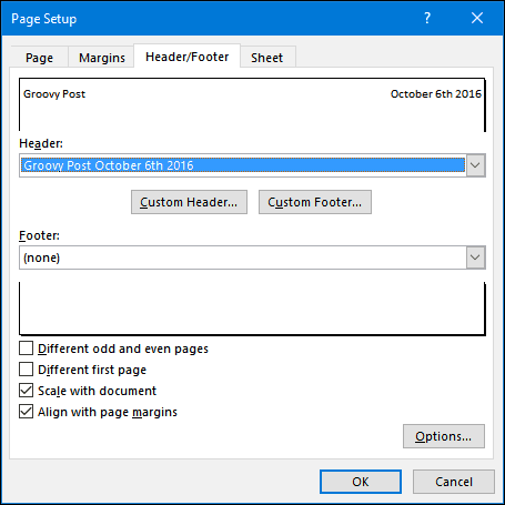
If you can’t get all the data on one page, use the Page Setup dialog to make further adjustments. The scaling menu can help you reduce the size of text to help it fit better. Try not to scale too much, since you want to keep text legible.

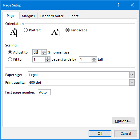
You can also use the same dialog to dress up your spreadsheet with a header and footer if desired.