Open Orders -Excel Report (SLSOPORDRP)

Can be accessed by:

1. Menu 51855

This gives you detailed instructions how to use the Open Orders Excel Report. This report can give you limitless options on what data you want to see on the Open Orders Report. This can be customized in so many different ways, that this guide has been requested to explain all of the options.

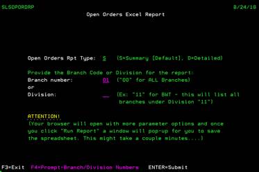
This report gives you access to the open orders currently in the system. This Open Order Report can be customized in any fashion you desire. From this screen, you can FILTER the Open Order report by Branch or Division number. If you do not know the branch number or division number, you can press F4 while on these fields to see the lookup features. You can also choose to have a Summary Report or the Detailed Report. Once your filter and report type have been selected and you have pressed ENTER, the search process begins. Please note, this program reviews all orders in the system to check for the current order status. This process can take several minutes. The report results are well worth the wait.

Open Orders Excel Report (Branchlookup)

Can be accessed by:

1. Menu 51855, F4 on branch field

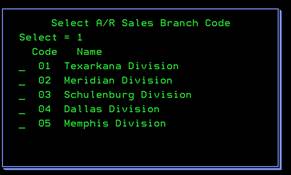
While on the Open Order screen, you can select to filter by Branch number. If you do not know the branch number, you can press F4 while on this field to see the lookup feature. While the popup box is on the screen, you can use “1” to select the appropriate branch and press ENTER. If the branch isn’t shown, press PAGE DOWN to view the remaining choices.

Open Orders Excel Report (Divisionlookup)

Can be accessed by:

1. Menu 51855, F4 on division field

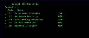
While on the Open Order screen, you can select to filter by Division number. All branches under the division will be shown on your report. If you do not know the division number, you can press F4 while on this field to see the lookup feature. While the popup box is on the screen, you can use “1” to select the appropriate division and press ENTER. If the division isn’t shown, press PAGE DOWN to view the remaining choices.

Web Query Filter (DB2WEBQUERY)

Can be accessed by:

1. Menu 51855, complete filter selections, ENTER

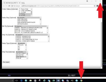
After the branch/division filter and report type have been selected, a new window pops up in the Chrome web browser. Additional filters are available to further customize your Open Order report. These six filters are optional. However, if you do not make any selections in these filters, your report will be larger and take more time accordingly. Selecting items in these filters are explained below.

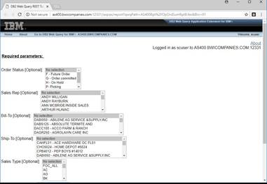
You can choose one, two, or more filter options to customize your report. On each of the filters you can choose one or more of the scroll down options that you want to appear on your report. The six filters are:

1. Order Status (future, order committed, on hold, picking, in pool or any combination)

2. Sales Rep (choose a single salesman or any combination)

3. Bill-To (can choose a single customer or any combination)

4. Ship-To (can choose a single customer or any combination)

5. Sales Type (FOC_ALL, AC, AO, BK, CC, CI, CO, DC, DS, IC, RS, SD, SF, SY, WC, WI, WO or any combination)

6. Ship Via (Motor Frt, Our Truck, Pickup, Post Office, UPS 3 day, UPS Ground, UPS no chrge, WC express, WC Exps Truck, WC Telephone, WC walk-in or any combination)

With all these options available, you can customize this report a different way each time you run this report. Here are some report examples:

A. If you want just the “On Hold” orders, click on that option only. It should be highlighted in BLUE to show it is selected.

B. If you want to select multiple items in one filter (example: both Picking and In Pool statuses), hold down the CTRL key and click all of your selections. They should all be highlighted in BLUE.

C. If you do not select an item in that filter option, all statuses listed will be included on your report.

D. If you want all “On Hold” orders for all salesmen that are going by “Our Truck”, you can select just those options in the filters and make those selections.

E. If a salesman was scheduled for vacation and wanted to see all of his customers’ Open Orders, he could select only his name in the Sales Rep filter and no other selections are necessary.

These filters help to personally select the data you are looking for at any given time. These six options make your Open Orders Report not only unique, but flexible each time you run the report.

Once you have completed your filter selections, press ENTER. You will see the following message at the bottom of your Chrome Web browser:

Depending on your selections, the report will filter through all open orders to bring back only the data you requested. Once the report is ready, you will see the following at the bottom of the Chrome Web Browser:

Simply ‘Click’ on the Excel symbol and the Open Order Report Excel Spreadsheet will open for viewing and further manipulation.

Open Order Excel Spreadsheet (OPORDSUMRPTB)

Can be accessed by:

1. Menu 51855, complete filter selections, ENTER, Chrome filters selected

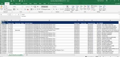
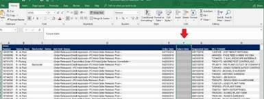
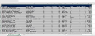
You are now viewing your Open Order Excel report. Once you are in Excel, you can manipulate this report in whatever fashion you need. You have 18 columns of data. These include everything from: order#, order date, bill to name, sales rep, ship via, goods total and sales type.

Altering your Excel Spreadsheet

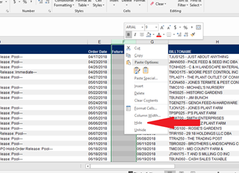
Hiding Columns:

If you wish to eliminate a column, simply “click” on the LETTER above the column you wish to remove. The column LETTER should change colors and the entire column should be selected.

After the column is highlighted, press the “right click” button on your mouse to pull up options. Among these options should be “Hide”. Click on this option to HIDE the highlighted column from the current view. It is suggested to HIDE the column instead of deleting it. You can always go back and “Unhide” a column to bring it back into view. You cannot “undelete” a column once you have saved the file after its deletion.

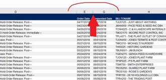
When you HIDE a column, the column LETTER will not show up at the top list anymore. It will show a gap between the surrounding columns. This is how Excel lets you know a hidden column exists in the event you want to “Unhide” the column later.

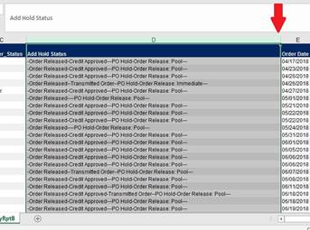
Alter Column Size:

If you wish to shorten the width of a column, simply click on the LETTER of the column you wish to shorten. Once the column is highlighted, “click” on the ’|’ column border line. You can drag to shorten or lengthen any column once you click on the border line of a column.

Sorting:

If you noticed, the report automatically sorts by the Order Number in Ascending order. If you wish to sort on another column, you can follow these steps: Hold down the CTRL button and at the same time press ‘A’. This will select ALL items on the spreadsheet. The entire spreadsheet should be highlighted.

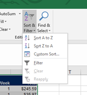
Click on the Sort & Filter Icon on the Excel Menu and choose Custom Sort from the popup box.

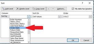
A selection window appears to help you choose which columns you wish to sort on. If you want to sort by “Order Date” for example, click the down arrow on SORT BY column and select, “Order Date” and click OK. You can sort on any column or even multiple columns if desired.

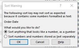
If the column’s data has data that Excel isn’t sure about, it may ask you about sorting data as a number or as text. We are going to sort as numbers for the Order Date.

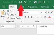
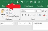
Saving your spreadsheet:

Once you have designed the Excel Spreadsheet into the report you need, save this report by clicking on the SAVE icon or by choosing FILE and then SAVE AS. Give your spreadsheet an appropriate name and save where you can readily find it later.

Exiting the Open Orders Report

Once you have completed your report save, be sure to close out the Chrome Web browser by clicking on the Chrome Icon on the bottom of your screen. Once the Chrome browser reappears, then click the ‘X’ in the upper right-hand corner.